Getting Started with R and RStudio

UQ Building

Introduction

This tutorial introduces R and RStudio — the programming language and development environment used throughout LADAL. It is aimed at complete beginners with no prior programming experience, and walks through everything you need to get up and running: installing software, understanding the RStudio interface, setting up a reproducible project, and working with R for the first time.

R is a free, open-source programming language designed specifically for data analysis and statistics. It is the most widely used tool for quantitative research in linguistics, the social sciences, and the digital humanities — and for good reason. R gives you complete control over your analysis, produces publication-quality graphics, and keeps your work fully transparent and reproducible.

This tutorial will not turn you into an expert. Its goal is to give you a solid, well-structured foundation: to know where things are, how to think about R, and how to start doing real things with data. The rest of LADAL’s tutorials build from here.

Prerequisite Tutorials

This tutorial has no prerequisites — it is designed for complete beginners. However, the following background tutorials are helpful companions:

• Introduction to Quantitative Reasoning
  
• Basic Concepts in Quantitative Research
  
• Reproducible Research
  

What This Tutorial Covers

1. Installing R and RStudio — getting everything set up on your computer
   
2. The RStudio interface — understanding the four panes and how to navigate them
   
3. R Projects and R Notebooks — setting up reproducible, well-organised workflows
   
4. R fundamentals — objects, functions, operators, and data types
   
5. Data structures — vectors, data frames, lists, and factors
   
6. Indexing and subsetting — accessing and filtering data
   
7. Working with data — loading, inspecting, and manipulating tabular data
   
8. Basic visualisation — creating your first plots with ggplot2
   
9. Getting help — where to turn when things go wrong
   

Citation

Martin Schweinberger. 2026. Getting Started with R and RStudio. The Language Technology and Data Analysis Laboratory (LADAL), The University of Queensland, Australia. url: https://ladal.edu.au/tutorials/intror/intror.html (Version 2026.03.27), doi: .

---

Why R?

Before diving in, it is worth briefly explaining why R is worth learning.

R is free and open-source — there are no licensing costs, ever. It is the dominant tool for statistical analysis in linguistics, psychology, and the social sciences. It has a vast ecosystem of over 20,000 contributed packages that extend its capabilities to cover almost any analytical task imaginable. Its reproducibility features — the ability to combine code, output, and prose in a single document — mean your analyses can be fully transparent and re-run by anyone. And its visualisation capabilities, particularly through ggplot2, are unmatched.

The learning curve is real but manageable. This tutorial gives you the foundation you need.

---

Preparation and Session Set-up

Install the packages used in this tutorial (only needed once):

install.packages("dplyr")  
install.packages("ggplot2")  
install.packages("tidyr")  
install.packages("flextable")  
install.packages("readxl")  
install.packages("here")  
install.packages("checkdown")  

Load the packages at the start of each session:

library(dplyr)       # data manipulation  
library(ggplot2)     # data visualisation  
library(tidyr)       # data reshaping  
library(flextable)   # formatted tables  
library(here)        # robust file paths  
library(checkdown)   # interactive exercises  

---

Installing R and RStudio

Section Overview

What you’ll learn: How to install R and RStudio on your computer

Why it matters: You need both installed to follow any LADAL tutorial

Time: ~15–30 minutes (mostly waiting for downloads)

R and RStudio are two separate pieces of software that work together. Think of R as the engine and RStudio as the car — you need both, and you interact almost exclusively with RStudio.

Installing R

R must be installed before RStudio. Visit cran.r-project.org and select the download for your operating system:

• Windows: click Download R for Windows → base → Download R x.x.x for Windows
  
• Mac: click Download R for macOS → select the version matching your macOS
  
• Linux: follow the instructions for your distribution

Run the downloaded installer and accept the default settings throughout.

Keeping R Up to Date

R releases a new version approximately once a year. To check your current version, run R.version$version.string in the console. To update on Windows, the installr package automates the process:

install.packages("installr")  
library(installr)  
updateR()  

On Mac, download the new version from CRAN and install over the existing version.

Installing RStudio

Visit posit.co/download/rstudio-desktop and download the free RStudio Desktop version for your operating system. Run the installer and accept the defaults.

After installation, open RStudio (not R directly). RStudio will automatically detect your R installation.

---

The RStudio Interface

Section Overview

What you’ll learn: How to navigate the four panes of RStudio and what each one does

Key concept: The difference between the Console (run immediately) and the Script Editor (save and reuse)

When you first open RStudio, you will see an interface divided into panes. The screenshot below shows a typical RStudio session with all four panes visible.

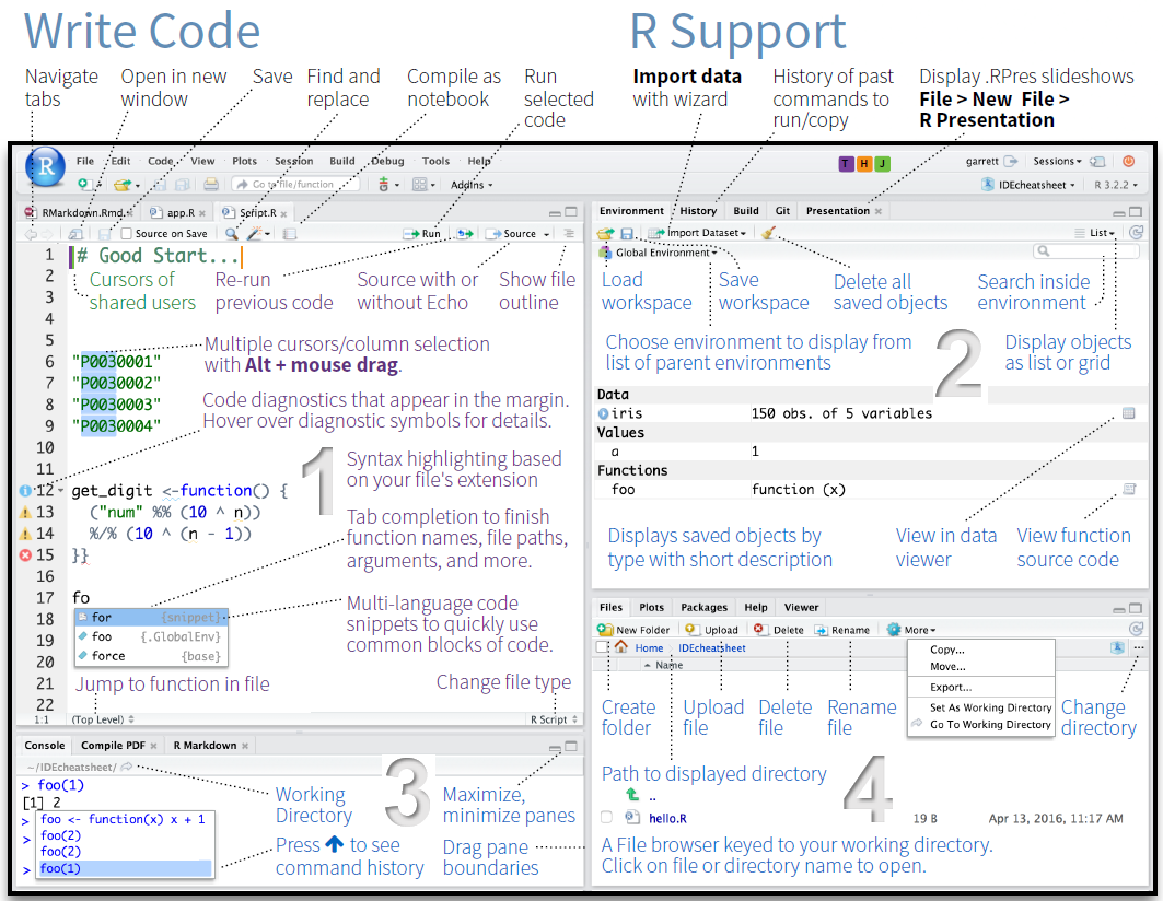
RStudio has four main panes:

Pane 1: Script Editor (top left)

This is where you write and save code. Code typed here does not run automatically — you must explicitly execute it. This is where all your analysis lives.

To run a line of code from the Script Editor, place your cursor on that line and press Ctrl + Enter (Windows/Linux) or Cmd + Enter (Mac). To run a highlighted block, select the code first and then press the same shortcut.

Pane 2: Console (bottom left)

This is where R executes code and displays text output. When you run code from the Script Editor, it appears here. You can also type directly into the Console and press Enter to run commands immediately.

Use the Console for quick experiments. Use the Script Editor for anything you want to keep.

Console Shortcuts

• Press the Up arrow in the Console to recall previous commands
  
• Type the beginning of a command and press Tab to autocomplete
  
• Type ?function_name to open the help page for any function
  

Pane 3: Environment and History (top right)

The Environment tab shows all objects currently loaded in your R session — data frames, variables, vectors, and so on. Clicking on a data frame here opens a spreadsheet-style viewer.

The History tab logs all commands you have run in the current session.

Pane 4: Files, Plots, Help, Packages (bottom right)

This multi-tab pane contains:

• Files: Browse your project folder
  
• Plots: View graphics output here
  
• Help: Documentation for functions and packages (also accessible via ?)
  
• Packages: See which packages are installed and loaded
  
• Viewer: Preview rendered documents

---

Projects and Notebooks

Section Overview

What you’ll learn: How to set up a reproducible project in RStudio; what an R Notebook is and why to use one

Key concept: An R Project keeps all your files, code, and data together in one self-contained folder

Good organisation before you start coding saves a great deal of trouble later. This section walks through the recommended setup.

Step 1: Create a Project Folder

Before opening RStudio, create a folder on your computer for your project. Inside it, create the following sub-folders:

my_project/  
├── data/          ← raw and processed data files  
├── images/        ← figures saved from R  
├── tables/        ← tables exported from R  
└── docs/          ← notes, reports, and output documents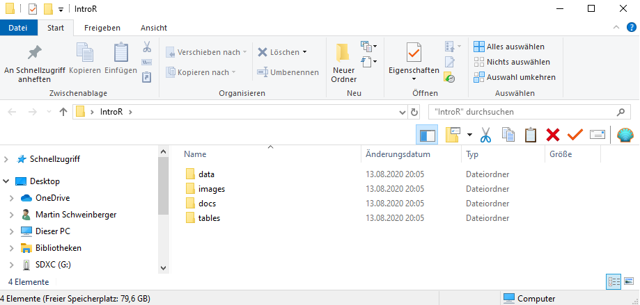  

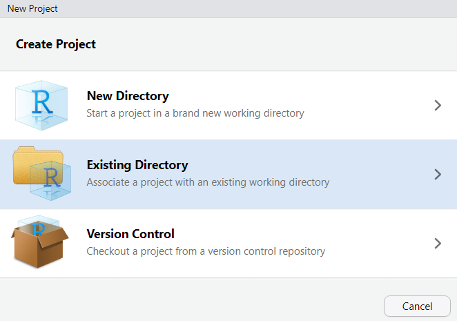
Step 2: Create an R Project

An R Project tells RStudio that a folder is a self-contained project. It sets the working directory automatically (so file paths are predictable) and keeps your project’s history and settings separate from other projects.

To create an R Project:

1. Open RStudio
   
2. Click File → New Project
   
3. Select Existing Directory
   
4. Navigate to your project folder and click Create Project

RStudio will restart and you will see your project name in the top-right corner. You are now working inside your project.

Always Work Inside an R Project

When you open RStudio, always open your project first (either by double-clicking the .Rproj file in your folder, or via File → Open Project). This ensures file paths work correctly and your environment is isolated.

Step 3: Create an R Notebook

An R Notebook (.Rmd or .qmd file) combines prose, code, and output in a single document. This is the standard format for LADAL tutorials and is highly recommended for your own analyses — it keeps your thinking and your code together.

To create an R Notebook:

1. Click File → New File → R Notebook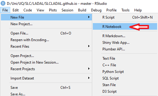
   
2. Give it a meaningful title
   
3. Save it in your project folder

The notebook uses R Markdown — a simple formatting syntax explained below.

R Markdown Basics

R Markdown lets you write formatted prose alongside executable code. Here is a quick reference:

# Heading 1  
## Heading 2  
### Heading 3  
  
**bold text**  
*italic text*  
`inline code`  
  
- bullet point  
- another bullet  
  
1. numbered item  
2. another item  
  
[link text](https://url.com)  

Code is written inside code chunks (fenced with triple backticks):

::: {.cell}

```{.r .cell-code}
# your R code here  
2 + 2  
```

::: {.cell-output .cell-output-stdout}

```
[1] 4
```


:::
:::

When you click Knit (or Render in Quarto), R Markdown executes all code chunks and weaves the output together with your prose into a finished HTML, PDF, or Word document.

Reproducibility

The power of R Notebooks is reproducibility: your entire analysis — every number, table, and figure — is regenerated from scratch each time you render the document. Anyone with your .Rmd file and data can reproduce your results exactly.

---

R Fundamentals

Section Overview

What you’ll learn: The core building blocks of R — objects, functions, operators, and assignment

Key concepts: Everything in R is an object; everything you do in R uses a function

Setting Up a Session

At the top of any script or notebook, set global options and load packages. This makes your session reproducible from the very first line.

# Global options  
options(stringsAsFactors = FALSE)   # keep character variables as text  
options(scipen = 100)               # avoid scientific notation  
options(max.print = 100)            # limit printed output  
  
# Load packages  
library(dplyr)  
library(ggplot2)  

Objects and Assignment

In R, everything is stored as an object. You create objects using the assignment operator <-:

# Create a numeric object  
my_number <- 42  
  
# Create a character (text) object  
my_name <- "linguistics"  
  
# Create a logical object  
is_true <- TRUE  
  
# View an object by typing its name  
my_number  

[1] 42

my_name  

[1] "linguistics"

is_true  

[1] TRUE

Naming Objects

Good object names are:
- lowercase with underscores for spaces: word_count, not Word Count
- descriptive: reaction_time_ms is better than x
- not starting with a number: data1 is valid; 1data is not
- not reserved words: don’t use c, t, df, mean, TRUE, FALSE, NULL as object names

R is case-sensitive: MyData and mydata are different objects.

Functions

A function takes one or more inputs (called arguments), does something, and returns an output. Functions are called by name followed by parentheses containing the arguments:

# sqrt() takes a number and returns its square root  
sqrt(144)  

[1] 12

# round() rounds a number to a specified number of decimal places  
round(3.14159, digits = 2)  

[1] 3.14

# nchar() counts the characters in a string  
nchar("linguistics")  

[1] 11

# paste() joins strings together  
paste("language", "data", "analysis", sep = "-")  

[1] "language-data-analysis"

You can nest functions — the inner function runs first:

# Round the square root of 2 to 3 decimal places  
round(sqrt(2), digits = 3)  

[1] 1.414

Operators

R provides standard arithmetic and logical operators:

# Arithmetic operators  
10 + 3    # addition  

[1] 13

10 - 3    # subtraction  

[1] 7

10 * 3    # multiplication  

[1] 30

10 / 3    # division  

[1] 3.333333

10 ^ 2    # exponentiation  

[1] 100

10 %% 3   # modulo (remainder)  

[1] 1

# Comparison operators (return TRUE or FALSE)  
5 > 3     # greater than  

[1] TRUE

5 < 3     # less than  

[1] FALSE

5 == 5    # equal to (note: double equals!)  

[1] TRUE

5 != 3    # not equal to  

[1] TRUE

5 >= 5    # greater than or equal to  

[1] TRUE

# Logical operators  
TRUE & FALSE   # AND  

[1] FALSE

TRUE | FALSE   # OR  

[1] TRUE

!TRUE          # NOT  

[1] FALSE

= vs ==

One of the most common beginner errors: = is used for assignment (interchangeable with <- in most cases, though <- is preferred); == tests whether two things are equal. 5 = 3 will produce an error; 5 == 3 returns FALSE.

---

Exercises: R Fundamentals

Q1. What does the assignment operator <- do?

It tests whether two values are equal
It calls a function with the specified argument
It subtracts the right-hand value from the left-hand value
It creates an object by storing a value under a name in the current environment

---

Q2. You run my_var <- 10. What will my_var * 3 + 1 return?

31
30
13
An error, because my_var is not a function

---

Q3. Which of the following is NOT a valid object name in R?

2nd_group
group_2
group.two
myGroup

---

Data Types

Section Overview

What you’ll learn: The six basic data types in R and why they matter

Key concept: The type of your data determines which operations are valid

Every object in R has a type (also called a class). The four types you will encounter most often are:

# Numeric (continuous numbers)  
age <- 28.5  
class(age)  

[1] "numeric"

# Integer (whole numbers; the L suffix forces integer type)  
count <- 42L  
class(count)  

[1] "integer"

# Character (text; always in quotes)  
language <- "English"  
class(language)  

[1] "character"

# Logical (TRUE or FALSE only)  
is_native <- TRUE  
class(is_native)  

[1] "logical"

You can check the type of any object with class() or typeof(), and test for specific types:

is.numeric(age)  

[1] TRUE

is.character(language)  

[1] TRUE

is.logical(is_native)  

[1] TRUE

You can convert between types using coercion functions:

# Character to numeric  
as.numeric("3.14")  

[1] 3.14

# Numeric to character  
as.character(42)  

[1] "42"

# Numeric to logical (0 = FALSE, everything else = TRUE)  
as.logical(0)  

[1] FALSE

as.logical(1)  

[1] TRUE

as.logical(-99)  

[1] TRUE

Coercion Failures

When R cannot coerce a value, it introduces NA (missing value) with a warning:

as.numeric("hello")  # "hello" cannot be a number → NA  

Warning: NAs introduced by coercion

[1] NA

NA stands for Not Available and represents missing data. It propagates through calculations — any arithmetic involving NA returns NA unless specifically handled.

---

Data Structures

Section Overview

What you’ll learn: How R organises collections of data — vectors, data frames, lists, and factors

Key concept: Vectors are the fundamental unit; data frames are collections of equal-length vectors

Vectors

A vector is a sequence of values of the same type. Vectors are created with c() (short for combine):

# Numeric vector  
word_lengths <- c(3, 5, 2, 8, 4, 6, 1)  
  
# Character vector  
languages <- c("English", "German", "Mandarin", "Arabic")  
  
# Logical vector  
is_content_word <- c(TRUE, TRUE, FALSE, TRUE, FALSE)  

You can perform operations on entire vectors at once — R applies them element-by-element:

# Arithmetic on a vector  
word_lengths * 2  

[1]  6 10  4 16  8 12  2

# Logical comparison on a vector  
word_lengths > 4  

[1] FALSE  TRUE FALSE  TRUE FALSE  TRUE FALSE

# Common summary functions  
length(word_lengths)     # number of elements  

[1] 7

sum(word_lengths)        # sum  

[1] 29

mean(word_lengths)       # mean  

[1] 4.142857

sd(word_lengths)         # standard deviation  

[1] 2.410295

min(word_lengths)        # minimum  

[1] 1

max(word_lengths)        # maximum  

[1] 8

range(word_lengths)      # min and max together  

[1] 1 8

Sequences and Repetitions

# Create a sequence with :  
1:10  

 [1]  1  2  3  4  5  6  7  8  9 10

# Create a sequence with seq()  
seq(from = 0, to = 1, by = 0.25)  

[1] 0.00 0.25 0.50 0.75 1.00

seq(from = 1, to = 100, length.out = 5)  

[1]   1.00  25.75  50.50  75.25 100.00

# Repeat values with rep()  
rep("yes", times = 3)  

[1] "yes" "yes" "yes"

rep(c("A", "B"), times = 4)  

[1] "A" "B" "A" "B" "A" "B" "A" "B"

rep(c("A", "B"), each = 4)  

[1] "A" "A" "A" "A" "B" "B" "B" "B"

Factors

A factor is a special type of vector for categorical variables. Factors have a fixed set of levels (categories) and are essential for grouping in analyses and plots.

# Create a factor  
register <- factor(c("Formal", "Informal", "Formal", "ReadAloud", "Informal"))  
  
# Inspect the factor  
register  

[1] Formal    Informal  Formal    ReadAloud Informal 
Levels: Formal Informal ReadAloud

levels(register)    # the unique categories  

[1] "Formal"    "Informal"  "ReadAloud"

nlevels(register)   # how many categories  

[1] 3

table(register)     # frequency of each level  

register
   Formal  Informal ReadAloud 
        2         2         1 

By default, levels are ordered alphabetically. You can specify a custom order:

# Custom level order (important for plots and models)  
register_ordered <- factor(  
  c("Formal", "Informal", "Formal", "ReadAloud", "Informal"),  
  levels = c("Formal", "ReadAloud", "Informal")  
)  
  
levels(register_ordered)  

[1] "Formal"    "ReadAloud" "Informal" 

Data Frames

A data frame is R’s equivalent of a spreadsheet — a table where each column is a vector of the same length. Data frames are the most common way to store linguistic data.

# Create a data frame from scratch  
speakers <- data.frame(  
  ID          = 1:6,  
  Name        = c("Alice", "Bob", "Carol", "David", "Eve", "Frank"),  
  L1          = c("English", "German", "English", "Mandarin", "English", "Arabic"),  
  Age         = c(24, 31, 28, 22, 35, 27),  
  Proficiency = factor(c("Advanced", "Intermediate", "Advanced",  
                          "Beginner", "Intermediate", "Advanced"),  
                       levels = c("Beginner", "Intermediate", "Advanced"))  
)  
  
# Inspect the data frame  
speakers  

  ID  Name       L1 Age  Proficiency
1  1 Alice  English  24     Advanced
2  2   Bob   German  31 Intermediate
3  3 Carol  English  28     Advanced
4  4 David Mandarin  22     Beginner
5  5   Eve  English  35 Intermediate
6  6 Frank   Arabic  27     Advanced

Key functions for inspecting a data frame:

nrow(speakers)         # number of rows (observations)  

[1] 6

ncol(speakers)         # number of columns (variables)  

[1] 5

dim(speakers)          # both at once  

[1] 6 5

names(speakers)        # column names  

[1] "ID"          "Name"        "L1"          "Age"         "Proficiency"

str(speakers)          # structure: types and first values  

'data.frame':   6 obs. of  5 variables:
 $ ID         : int  1 2 3 4 5 6
 $ Name       : chr  "Alice" "Bob" "Carol" "David" ...
 $ L1         : chr  "English" "German" "English" "Mandarin" ...
 $ Age        : num  24 31 28 22 35 27
 $ Proficiency: Factor w/ 3 levels "Beginner","Intermediate",..: 3 2 3 1 2 3

head(speakers, n = 3)  # first 3 rows  

  ID  Name      L1 Age  Proficiency
1  1 Alice English  24     Advanced
2  2   Bob  German  31 Intermediate
3  3 Carol English  28     Advanced

tail(speakers, n = 2)  # last 2 rows  

  ID  Name      L1 Age  Proficiency
5  5   Eve English  35 Intermediate
6  6 Frank  Arabic  27     Advanced

summary(speakers)      # summary statistics per column  

       ID           Name                L1                 Age       
 Min.   :1.00   Length:6           Length:6           Min.   :22.00  
 1st Qu.:2.25   Class :character   Class :character   1st Qu.:24.75  
 Median :3.50   Mode  :character   Mode  :character   Median :27.50  
 Mean   :3.50                                         Mean   :27.83  
 3rd Qu.:4.75                                         3rd Qu.:30.25  
 Max.   :6.00                                         Max.   :35.00  
       Proficiency
 Beginner    :1   
 Intermediate:2   
 Advanced    :3   
                  
                  
                  

Lists

A list is the most flexible data structure — it can hold objects of different types and lengths, including other lists.

# Create a list with mixed types  
my_list <- list(  
  name     = "Study 1",  
  n        = 30,  
  groups   = c("Control", "Treatment"),  
  complete = TRUE  
)  
  
# Access list elements with $ or [[]]  
my_list$name  

[1] "Study 1"

my_list[["n"]]  

[1] 30

Lists are commonly returned by statistical model functions (e.g., lm() returns a list). You rarely create them from scratch but frequently need to extract elements from them.

---

Exercises: Data Structures

Q1. You run x <- c(1, 2, "three", 4). What type will x be?

Numeric — the numbers override the character
It produces an error because you cannot mix types in a vector
Character — R coerces all elements to the most flexible type that can represent all values
Mixed — R keeps each element as its original type

---

Q2. What is the difference between a factor and a character vector?

A factor has a fixed set of predefined levels (categories); a character vector is just text with no inherent structure
Character vectors are faster to compute with than factors
There is no practical difference — they behave identically
Factors can only contain numbers; character vectors contain text

---

Q3. What does dim(df) return for a data frame with 50 rows and 4 columns?

200 — the total number of cells
c(50, 4) — a vector with number of rows first, then number of columns
c(4, 50) — columns first, then rows
A list with named elements $rows and $cols

---

Indexing and Subsetting

Section Overview

What you’ll learn: How to access specific elements, rows, columns, and subsets of your data

Key concept: Square brackets [ ] select by position; $ selects columns by name; dplyr verbs filter by condition

Extracting exactly the data you need is one of the most fundamental R skills.

Indexing Vectors

Use square brackets [ ] with a position number (index) to extract elements from a vector. R indexing starts at 1 (not 0 as in Python).

languages <- c("English", "German", "Mandarin", "Arabic", "French")  
  
# Extract a single element  
languages[1]       # first element  

[1] "English"

languages[4]       # fourth element  

[1] "Arabic"

# Extract multiple elements  
languages[c(1, 3)] # first and third  

[1] "English"  "Mandarin"

languages[2:4]     # second through fourth  

[1] "German"   "Mandarin" "Arabic"  

# Exclude elements (negative indexing)  
languages[-2]      # everything except the second element  

[1] "English"  "Mandarin" "Arabic"   "French"  

languages[-c(1,5)] # everything except first and fifth  

[1] "German"   "Mandarin" "Arabic"  

# Logical indexing  
word_lengths <- c(3, 5, 2, 8, 4, 6, 1)  
word_lengths[word_lengths > 4]          # elements greater than 4  

[1] 5 8 6

word_lengths[word_lengths == min(word_lengths)]  # the minimum value  

[1] 1

Indexing Data Frames

Data frames have two dimensions: df[row, column]. Leave one blank to select all rows or all columns.

# Using the speakers data frame from earlier  
  
# Single cell: row 2, column 3  
speakers[2, 3]  

[1] "German"

# Entire row 1  
speakers[1, ]  

  ID  Name      L1 Age Proficiency
1  1 Alice English  24    Advanced

# Entire column 3 (returns a vector)  
speakers[, 3]  

[1] "English"  "German"   "English"  "Mandarin" "English"  "Arabic"  

# Column by name using $  
speakers$Age  

[1] 24 31 28 22 35 27

speakers$L1  

[1] "English"  "German"   "English"  "Mandarin" "English"  "Arabic"  

# Multiple rows and columns  
speakers[1:3, c("Name", "Age")]  

   Name Age
1 Alice  24
2   Bob  31
3 Carol  28

Subsetting with dplyr

While base R indexing works, the dplyr package provides cleaner, more readable syntax for filtering and selecting data. These are the two most important dplyr verbs for subsetting:

# filter() keeps rows that meet a condition  
speakers |>  
  dplyr::filter(L1 == "English")  

  ID  Name      L1 Age  Proficiency
1  1 Alice English  24     Advanced
2  3 Carol English  28     Advanced
3  5   Eve English  35 Intermediate

# select() keeps specified columns  
speakers |>  
  dplyr::select(Name, Age, Proficiency)  

   Name Age  Proficiency
1 Alice  24     Advanced
2   Bob  31 Intermediate
3 Carol  28     Advanced
4 David  22     Beginner
5   Eve  35 Intermediate
6 Frank  27     Advanced

# Combine both  
speakers |>  
  dplyr::filter(Age < 30) |>  
  dplyr::select(Name, L1, Age)  

   Name       L1 Age
1 Alice  English  24
2 Carol  English  28
3 David Mandarin  22
4 Frank   Arabic  27

The Pipe Operator |>

The pipe |> (from the magrittr/dplyr packages) passes the result on the left to the function on the right. It lets you chain operations in a readable left-to-right sequence instead of nesting functions:

# Without pipe (hard to read)  
select(filter(speakers, Age < 30), Name, Age)  
  
# With pipe (reads like a sentence)  
speakers |> filter(Age < 30) |> select(Name, Age)  

R 4.1+ also has a native pipe |> that works similarly. LADAL tutorials use |>.

---

Exercises: Indexing

Q1. Given v <- c(10, 20, 30, 40, 50), what does v[c(2, 4)] return?

20 40
10 30 50
2 4
An error

---

Q2. How do you use dplyr::filter() to keep only rows where the column Proficiency equals "Advanced"?

df[df$Proficiency = "Advanced", ]
df |> dplyr::filter(Proficiency == "Advanced")
df |> dplyr::filter(Proficiency = "Advanced")
df |> dplyr::select(Proficiency == "Advanced")

---

Working with Data

Section Overview

What you’ll learn: How to load data from files, inspect it, and perform common data manipulation operations

Key functions: read.csv(), readxl::read_excel(), dplyr::mutate(), dplyr::group_by(), dplyr::summarise()

Loading Data

From CSV

# Base R  
my_data <- read.csv("data/my_file.csv")  
  
# Using here() for robust paths (recommended)  
my_data <- read.csv(here::here("data", "my_file.csv"))  
  
# Tidyverse readr (slightly faster, better defaults)  
my_data <- readr::read_csv(here::here("data", "my_file.csv"))  

From Excel

library(readxl)  
my_data <- readxl::read_excel(here::here("data", "my_file.xlsx"))  
  
# Specify a sheet  
my_data <- readxl::read_excel(here::here("data", "my_file.xlsx"), sheet = "Sheet2")  

Saving Data

# Save as CSV  
write.csv(my_data, here::here("data", "processed_data.csv"), row.names = FALSE)  
  
# Save as R object (preserves factors and other R-specific attributes)  
saveRDS(my_data, here::here("data", "processed_data.rds"))  
  
# Load an RDS file  
my_data <- readRDS(here::here("data", "processed_data.rds"))  

Manipulating Data with dplyr

We will use a simulated linguistic dataset to demonstrate the key dplyr operations. The dataset contains reaction times and accuracy from a lexical decision task:

set.seed(42)  
n <- 60  
  
lex_data <- data.frame(  
  Participant    = rep(1:20, each = 3),  
  Condition      = rep(c("High_Freq", "Low_Freq", "Pseudoword"), times = 20),  
  RT_ms          = c(  
    rnorm(20, mean = 480, sd = 55),   # High frequency: fast  
    rnorm(20, mean = 610, sd = 70),   # Low frequency: slower  
    rnorm(20, mean = 730, sd = 80)    # Pseudowords: slowest  
  ),  
  Accurate       = sample(c(TRUE, FALSE), n, replace = TRUE, prob = c(0.9, 0.1))  
) |>  
  dplyr::mutate(Condition = factor(Condition,  
                                   levels = c("High_Freq", "Low_Freq", "Pseudoword")))  

mutate() — Add or Modify Columns

# Add a new column converting RT to seconds  
lex_data <- lex_data |>  
  dplyr::mutate(  
    RT_s         = RT_ms / 1000,  
    RT_log       = log(RT_ms),  
    Fast_respons = RT_ms < 500  
  )  
  
head(lex_data)  

  Participant  Condition    RT_ms Accurate      RT_s   RT_log Fast_respons
1           1  High_Freq 555.4027     TRUE 0.5554027 6.319693        FALSE
2           1   Low_Freq 448.9416     TRUE 0.4489416 6.106893         TRUE
3           1 Pseudoword 499.9721     TRUE 0.4999721 6.214552         TRUE
4           2  High_Freq 514.8074     TRUE 0.5148074 6.243793        FALSE
5           2   Low_Freq 502.2348     TRUE 0.5022348 6.219068        FALSE
6           2 Pseudoword 474.1632     TRUE 0.4741632 6.161551         TRUE

group_by() and summarise() — Aggregate by Group

lex_data |>  
  dplyr::group_by(Condition) |>  
  dplyr::summarise(  
    n          = n(),  
    M_RT       = round(mean(RT_ms), 1),  
    SD_RT      = round(sd(RT_ms), 1),  
    Accuracy   = round(mean(Accurate) * 100, 1),  
    .groups    = "drop"  
  ) |>  
  flextable() |>  
  flextable::set_table_properties(width = .8, layout = "autofit") |>  
  flextable::theme_zebra() |>  
  flextable::fontsize(size = 12) |>  
  flextable::fontsize(size = 12, part = "header") |>  
  flextable::align_text_col(align = "center") |>  
  flextable::set_caption(caption = "Reaction times and accuracy by condition in the lexical decision task.") |>  
  flextable::border_outer()  

Condition	n	M_RT	SD_RT	Accuracy
High_Freq	20	592.9	125.9	90
Low_Freq	20	605.0	117.9	80
Pseudoword	20	613.7	135.6	100

arrange() — Sort Rows

# Sort by RT (ascending)  
lex_data |>  
  dplyr::arrange(RT_ms) |>  
  head(5)  

  Participant  Condition    RT_ms Accurate      RT_s   RT_log Fast_respons
1           6 Pseudoword 333.8950     TRUE 0.3338950 5.810826         TRUE
2           7  High_Freq 345.7743     TRUE 0.3457743 5.845786         TRUE
3           5  High_Freq 403.6127     TRUE 0.4036127 6.000456         TRUE
4          13 Pseudoword 441.0055     TRUE 0.4410055 6.089057         TRUE
5           1   Low_Freq 448.9416     TRUE 0.4489416 6.106893         TRUE

# Sort descending  
lex_data |>  
  dplyr::arrange(desc(RT_ms)) |>  
  head(5)  

  Participant  Condition    RT_ms Accurate      RT_s   RT_log Fast_respons
1          18   Low_Freq 856.0582     TRUE 0.8560582 6.752338        FALSE
2          16 Pseudoword 845.5281     TRUE 0.8455281 6.739961        FALSE
3          15  High_Freq 790.6531     TRUE 0.7906531 6.672859        FALSE
4          19 Pseudoword 784.3431     TRUE 0.7843431 6.664847        FALSE
5          17   Low_Freq 782.4518     TRUE 0.7824518 6.662432        FALSE

rename() and relocate()

# Rename columns  
lex_data |>  
  dplyr::rename(ReactionTime = RT_ms, Correct = Accurate) |>  
  head(3)  

  Participant  Condition ReactionTime Correct      RT_s   RT_log Fast_respons
1           1  High_Freq     555.4027    TRUE 0.5554027 6.319693        FALSE
2           1   Low_Freq     448.9416    TRUE 0.4489416 6.106893         TRUE
3           1 Pseudoword     499.9721    TRUE 0.4999721 6.214552         TRUE

count() — Quick Frequency Tables

# How many observations per condition?  
lex_data |>  
  dplyr::count(Condition)  

   Condition  n
1  High_Freq 20
2   Low_Freq 20
3 Pseudoword 20

# Cross-tabulate condition and accuracy  
lex_data |>  
  dplyr::count(Condition, Accurate)  

   Condition Accurate  n
1  High_Freq    FALSE  2
2  High_Freq     TRUE 18
3   Low_Freq    FALSE  4
4   Low_Freq     TRUE 16
5 Pseudoword     TRUE 20

Handling Missing Values

# Check for missing values  
sum(is.na(lex_data$RT_ms))  

[1] 0

colSums(is.na(lex_data))  

 Participant    Condition        RT_ms     Accurate         RT_s       RT_log 
           0            0            0            0            0            0 
Fast_respons 
           0 

# Remove rows with any missing value  
lex_data_clean <- lex_data |>  
  tidyr::drop_na()  
  
# Replace NA with a value (e.g., mean imputation — use cautiously!)  
lex_data |>  
  dplyr::mutate(RT_ms = ifelse(is.na(RT_ms), mean(RT_ms, na.rm = TRUE), RT_ms))  

   Participant  Condition    RT_ms Accurate      RT_s   RT_log Fast_respons
1            1  High_Freq 555.4027     TRUE 0.5554027 6.319693        FALSE
2            1   Low_Freq 448.9416     TRUE 0.4489416 6.106893         TRUE
3            1 Pseudoword 499.9721     TRUE 0.4999721 6.214552         TRUE
4            2  High_Freq 514.8074     TRUE 0.5148074 6.243793        FALSE
5            2   Low_Freq 502.2348     TRUE 0.5022348 6.219068        FALSE
6            2 Pseudoword 474.1632     TRUE 0.4741632 6.161551         TRUE
7            3  High_Freq 563.1337    FALSE 0.5631337 6.333517        FALSE
8            3   Low_Freq 474.7938    FALSE 0.4747938 6.162881         TRUE
9            3 Pseudoword 591.0133     TRUE 0.5910133 6.381839        FALSE
10           4  High_Freq 476.5507     TRUE 0.4765507 6.166574         TRUE
11           4   Low_Freq 551.7678    FALSE 0.5517678 6.313127        FALSE
12           4 Pseudoword 605.7655     TRUE 0.6057655 6.406493        FALSE
13           5  High_Freq 403.6127     TRUE 0.4036127 6.000456         TRUE
14           5   Low_Freq 464.6666    FALSE 0.4646666 6.141320         TRUE
 [ reached 'max' / getOption("max.print") -- omitted 46 rows ]

---

Exercises: Working with Data

Q1. What does dplyr::mutate() do?

It adds new columns or modifies existing columns, keeping all other columns and rows unchanged
It removes rows that do not meet a condition
It summarises columns into a single value per group
It sorts the data frame by one or more columns

---

Q2. You want the mean RT for each participant across all conditions. Which dplyr pipeline is correct?

lex_data |> group_by(Participant) |> mutate(M_RT = mean(RT_ms))
lex_data |> summarise(M_RT = mean(RT_ms)) |> group_by(Participant)
lex_data |> group_by(Participant) |> summarise(M_RT = mean(RT_ms))
lex_data |> filter(Participant) |> mutate(M_RT = mean(RT_ms))

---

Basic Visualisation with ggplot2

Section Overview

What you’ll learn: How to create basic plots using ggplot2; the layered grammar of graphics

Key concept: Every ggplot2 plot is built by adding layers — data, aesthetics, geometries, and themes

ggplot2 is R’s most powerful and widely used plotting package. It is based on the Grammar of Graphics: the idea that every plot can be described by a consistent set of components.

The Grammar of Graphics

Every ggplot2 plot has at least three components:

1. Data: the data frame containing your variables
   
2. Aesthetics (aes()): which variables map to which visual properties (x axis, y axis, colour, size, shape)
   
3. Geometry (geom_*()): how the data are visually represented (points, bars, lines, boxes)

Additional optional components include scales, facets, themes, and labels.

ggplot(data = my_data, aes(x = variable1, y = variable2)) +  
  geom_point() +  
  theme_bw() +  
  labs(title = "My plot", x = "X label", y = "Y label")  

Histograms

ggplot(lex_data, aes(x = RT_ms, fill = Condition)) +  
  geom_histogram(bins = 20, color = "white", alpha = 0.7) +  
  facet_wrap(~ Condition, ncol = 1) +  
  scale_fill_manual(values = c("steelblue", "tomato", "seagreen")) +  
  theme_bw() +  
  theme(legend.position = "none", panel.grid.minor = element_blank()) +  
  labs(title = "Distribution of reaction times by condition",  
       x = "Reaction time (ms)", y = "Count")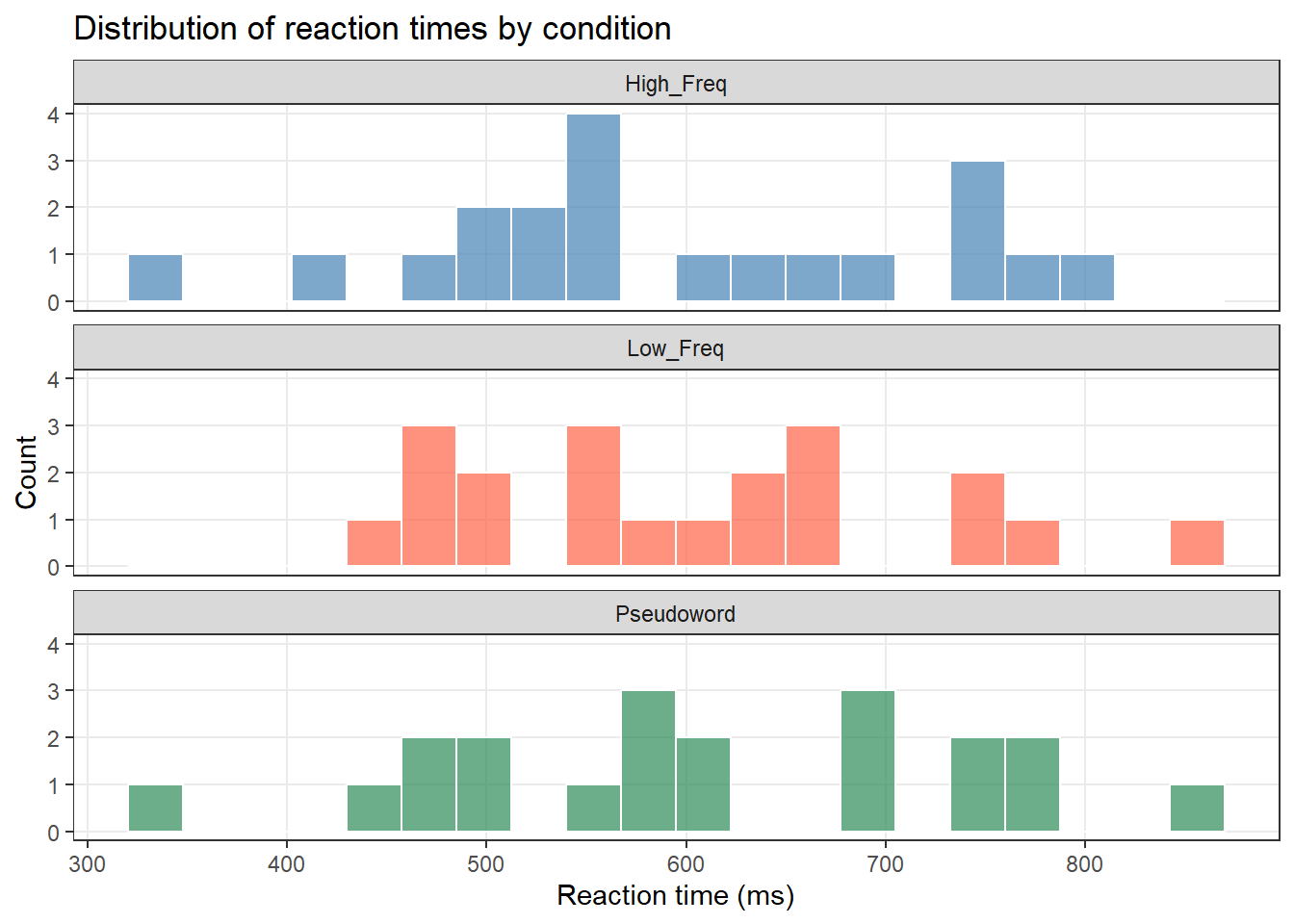  

Boxplots

ggplot(lex_data, aes(x = Condition, y = RT_ms, fill = Condition)) +  
  geom_boxplot(alpha = 0.7, outlier.color = "gray40") +  
  stat_summary(fun = mean, geom = "point",  
               shape = 18, size = 3, color = "black") +  
  scale_fill_manual(values = c("steelblue", "tomato", "seagreen")) +  
  theme_bw() +  
  theme(legend.position = "none", panel.grid.minor = element_blank()) +  
  labs(title = "Reaction times by condition",  
       subtitle = "Diamond = group mean; box = median and IQR",  
       x = "Condition", y = "Reaction time (ms)")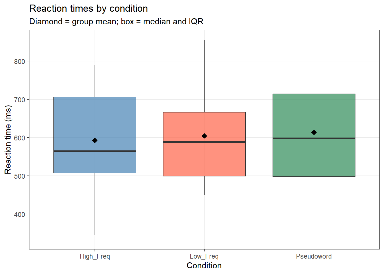  

Bar Charts

lex_data |>  
  dplyr::group_by(Condition) |>  
  dplyr::summarise(M_RT = mean(RT_ms),  
                   SE   = sd(RT_ms) / sqrt(n()),  
                   .groups = "drop") |>  
  ggplot(aes(x = Condition, y = M_RT, fill = Condition)) +  
  geom_col(alpha = 0.8, width = 0.6) +  
  geom_errorbar(aes(ymin = M_RT - SE, ymax = M_RT + SE),  
                width = 0.2, linewidth = 0.8) +  
  scale_fill_manual(values = c("steelblue", "tomato", "seagreen")) +  
  theme_bw() +  
  theme(legend.position = "none", panel.grid.minor = element_blank()) +  
  labs(title = "Mean reaction time by condition",  
       subtitle = "Error bars = ±1 SE",  
       x = "Condition", y = "Mean RT (ms)")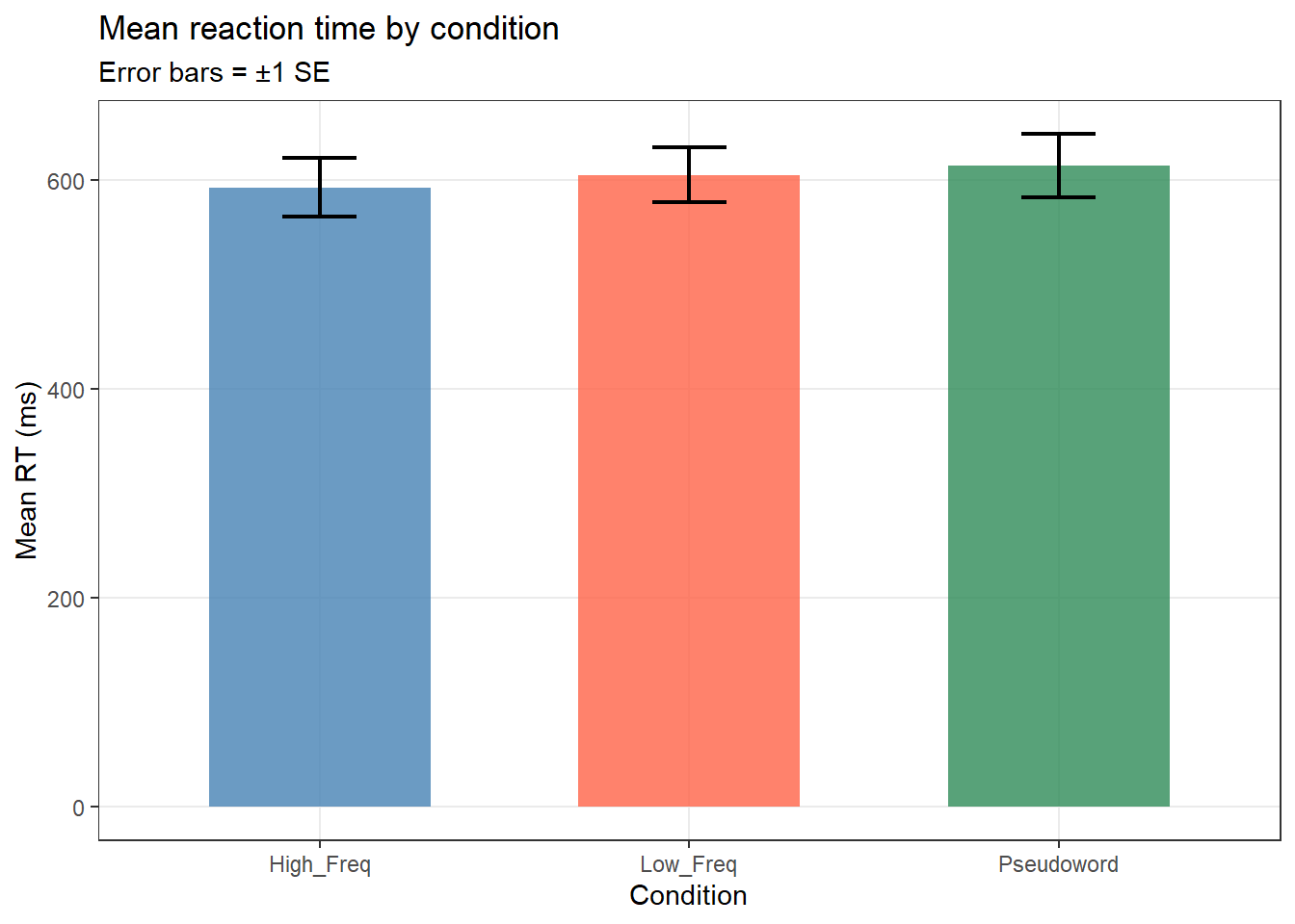  

Scatter Plots

ggplot(lex_data, aes(x = Participant, y = RT_ms, color = Condition)) +  
  geom_point(alpha = 0.7, size = 2) +  
  scale_color_manual(values = c("steelblue", "tomato", "seagreen")) +  
  theme_bw() +  
  theme(panel.grid.minor = element_blank()) +  
  labs(title = "Individual RT observations by participant and condition",  
       x = "Participant ID", y = "Reaction time (ms)",  
       color = "Condition")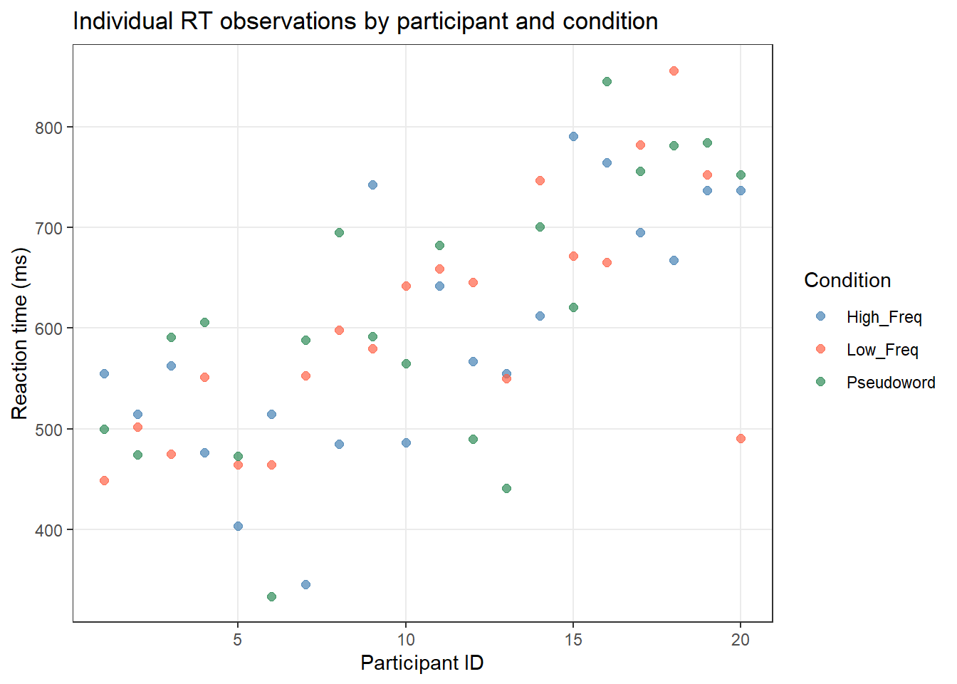  

Saving Plots

# Save the most recently displayed plot  
ggsave(  
  filename = here::here("images", "my_plot.png"),  
  width    = 8,  
  height   = 5,  
  dpi      = 300  
)  
  
# Save a named plot object  
my_plot <- ggplot(lex_data, aes(x = RT_ms)) + geom_histogram()  
  
ggsave(  
  plot     = my_plot,  
  filename = here::here("images", "histogram.pdf"),  
  width    = 6,  
  height   = 4  
)  

ggplot2 Quick Tips

• Add theme_bw() for a clean white background (LADAL standard)
  
• Add theme(panel.grid.minor = element_blank()) to remove minor gridlines
  
• Use scale_color_manual() / scale_fill_manual() to control colours
  
• Use facet_wrap(~ variable) to create small multiples
  
• Use labs() to set title, subtitle, and axis labels
  
• Use + coord_flip() to swap x and y axes (useful for long category names)
  

---

Exercises: Visualisation

Q1. In ggplot2, what does aes() control?

The type of plot geometry (e.g., histogram, boxplot, scatter)
The overall visual theme and background style
The mapping between variables in the data and visual properties of the plot (axes, colour, shape, size)
The axis labels and plot title

---

Q2. Which geom_*() function would you use to create a histogram?

geom_histogram()
geom_bar()
geom_col()
geom_density()

---

Getting Help

Section Overview

What you’ll learn: How to find help efficiently when you are stuck — both within R and online

Every R user gets stuck regularly. Knowing where to look for help is as important as knowing R itself.

Help Within R

# Help page for a specific function  
?mean  
help(mean)  
  
# Search for functions related to a keyword  
??regression  
apropos("filter")  
  
# See a function's arguments  
args(ggplot)  
  
# See examples of a function in action  
example(boxplot)  

RStudio’s Help tab (bottom right pane) renders help pages with formatted descriptions, argument lists, and examples.

Vignettes

Many packages include vignettes — detailed guides that show how to use the package end-to-end. These are often more useful than the function-level help pages:

# List all vignettes for a package  
vignette(package = "dplyr")  
  
# Open a specific vignette  
vignette("dplyr")  
vignette("ggplot2-specs")  

Reading Error Messages

Error messages are your friend — they tell you exactly what went wrong. Common error patterns:

Common Errors and What They Mean

object 'x' not found
→ The object x does not exist in your environment. Did you run the line that creates it? Is it spelled correctly (case-sensitive)?

could not find function "ggplot"
→ The package containing this function is not loaded. Did you run library(ggplot2)?

Error in read.csv("data.csv") : cannot open file
→ R cannot find the file. Check your working directory (getwd()), use here::here(), and check for typos in the filename.

non-numeric argument to binary operator
→ You tried to do arithmetic on a character string. Check the type of your object with class().

NAs introduced by coercion
→ R tried to convert a character to numeric but could not. The unconvertible values became NA. Inspect the affected column for unexpected text.

object of type 'closure' is not subsettable
→ You tried to index a function as if it were a data frame (e.g., mean[1]). Check whether you forgot parentheses somewhere.

Searching Online

The R community is enormous and helpful. When you encounter an error:

1. Copy the exact error message and paste it into Google with “R” at the start
   
2. Stack Overflow (stackoverflow.com) has answers to most common R questions
   
3. RStudio Community (community.rstudio.com) is welcoming to beginners
   
4. CRAN package pages list vignettes, reference manuals, and NEWS files
   
5. Package websites (e.g., dplyr.tidyverse.org) have well-structured guides

Writing a Good Question

If you need to ask for help, always provide:
- A minimal reproducible example — the smallest piece of code that demonstrates the problem
- Your session info: sessionInfo()
- The exact error message (copy-paste, do not retype)
- What you expected to happen vs. what actually happened

The reprex package helps format reproducible examples: install.packages("reprex")

Key Online Resources

Resource	URL	Why useful
R for Data Science	r4ds.hadley.nz	Free online book; the best comprehensive introduction to R and the tidyverse
RStudio Cheatsheets	posit.co/resources/cheatsheets	One-page quick references for popular packages (dplyr, ggplot2, RMarkdown, etc.)
CRAN Task Views	cran.r-project.org/web/views	Curated lists of R packages by topic (linguistics, NLP, spatial, etc.)
Stack Overflow [r]	stackoverflow.com/questions/tagged/r	Answers to nearly every R question; search before posting
Tidyverse documentation	tidyverse.org	Official documentation for dplyr, ggplot2, tidyr, readr, and more
ggplot2 documentation	ggplot2.tidyverse.org	Function reference, articles, and extension gallery
R Graph Gallery	r-graph-gallery.com	Hundreds of example plots with full reproducible code

---

Best Practices

Section Overview

What you’ll learn: Habits and conventions that make your R code more readable, reproducible, and robust

Good coding habits matter more the longer your projects become. These practices are worth building from day one.

Code Style

• Comment your code liberally: # This filters to English speakers only
  
• Use consistent naming: word_count not WordCount or wc
  
• Keep lines under 80 characters (use line breaks inside functions)
  
• Add spaces around operators: x <- 5 * (3 + 2) not x<-5*(3+2)
  
• Load all packages at the top of the script
  
• Set the random seed at the top when using random processes: set.seed(42)

Project Structure

• Always work inside an R Project (.Rproj)
  
• Use here::here() for all file paths — never hardcode absolute paths like "C:/Users/Martin/..."
  
• Keep raw data read-only — never overwrite original files; save processed versions separately
  
• Use version control (Git) for anything important

Reproducibility

• Write all analyses in R Notebooks or scripts — never rely on Console-only work
  
• Render your notebook from scratch periodically to confirm it runs end-to-end
  
• End every notebook with sessionInfo() to record package versions
  
• Consider using renv to snapshot your package environment

Environment Hygiene

# See all objects in your environment  
ls()  
  
# Remove a specific object  
rm(my_temp_variable)  
  
# Remove everything (use with caution!)  
rm(list = ls())  
  
# Check working directory  
getwd()  
  
# Change working directory (prefer R Projects over setwd())  
setwd("path/to/folder")  # avoid this; use R Projects instead  

Citation & Session Info

Citation

Martin Schweinberger. 2026. Getting Started with R and RStudio. The Language Technology and Data Analysis Laboratory (LADAL), The University of Queensland, Australia. url: https://ladal.edu.au/tutorials/intror/intror.html (Version 2026.03.27), doi: 10.5281/zenodo.19242479.

@manual{martinschweinberger2026getting,
  author       = {Martin Schweinberger},
  title        = {Getting Started with R and RStudio},
  year         = {2026},
  note         = {https://ladal.edu.au/tutorials/intror/intror.html},
  organization = {The Language Technology and Data Analysis Laboratory (LADAL), The University of Queensland, Australia},
  edition      = {2026.03.27}
  doi      = {10.5281/zenodo.19242479}
}

sessionInfo()  

R version 4.4.2 (2024-10-31 ucrt)
Platform: x86_64-w64-mingw32/x64
Running under: Windows 11 x64 (build 26200)

Matrix products: default


locale:
[1] LC_COLLATE=English_United States.utf8 
[2] LC_CTYPE=English_United States.utf8   
[3] LC_MONETARY=English_United States.utf8
[4] LC_NUMERIC=C                          
[5] LC_TIME=English_United States.utf8    

time zone: Australia/Brisbane
tzcode source: internal

attached base packages:
[1] stats     graphics  grDevices datasets  utils     methods   base     

other attached packages:
 [1] checkdown_0.0.13 flextable_0.9.7  here_1.0.1       tokenizers_0.3.0
 [5] tm_0.7-16        NLP_0.3-2        readxl_1.4.3     quanteda_4.2.0  
 [9] tidytext_0.4.2   lubridate_1.9.4  forcats_1.0.0    stringr_1.5.1   
[13] dplyr_1.2.0      purrr_1.0.4      readr_2.1.5      tidyr_1.3.2     
[17] tibble_3.2.1     ggplot2_4.0.2    tidyverse_2.0.0 

loaded via a namespace (and not attached):
 [1] fastmatch_1.1-6         gtable_0.3.6            xfun_0.56              
 [4] htmlwidgets_1.6.4       lattice_0.22-6          tzdb_0.4.0             
 [7] vctrs_0.7.1             tools_4.4.2             generics_0.1.3         
[10] parallel_4.4.2          janeaustenr_1.0.0       pkgconfig_2.0.3        
[13] Matrix_1.7-2            data.table_1.17.0       RColorBrewer_1.1-3     
[16] S7_0.2.1                uuid_1.2-1              lifecycle_1.0.5        
[19] compiler_4.4.2          farver_2.1.2            textshaping_1.0.0      
[22] codetools_0.2-20        litedown_0.9            fontLiberation_0.1.0   
[25] fontquiver_0.2.1        SnowballC_0.7.1         htmltools_0.5.9        
[28] yaml_2.3.10             pillar_1.10.1           openssl_2.3.2          
[31] fontBitstreamVera_0.1.1 commonmark_2.0.0        stopwords_2.3          
[34] zip_2.3.2               tidyselect_1.2.1        digest_0.6.39          
[37] stringi_1.8.4           slam_0.1-55             labeling_0.4.3         
[40] rprojroot_2.0.4         fastmap_1.2.0           grid_4.4.2             
[43] cli_3.6.4               magrittr_2.0.3          withr_3.0.2            
[46] gdtools_0.4.1           scales_1.4.0            timechange_0.3.0       
[49] officer_0.6.7           rmarkdown_2.30          cellranger_1.1.0       
[52] ragg_1.3.3              askpass_1.2.1           hms_1.1.3              
[55] evaluate_1.0.3          knitr_1.51              markdown_2.0           
[58] rlang_1.1.7             Rcpp_1.0.14             glue_1.8.0             
[61] xml2_1.3.6              renv_1.1.1              rstudioapi_0.17.1      
[64] jsonlite_1.9.0          R6_2.6.1                systemfonts_1.2.1      

AI Transparency Statement

This tutorial was written with the assistance of Claude (claude.ai), a large language model created by Anthropic. Claude was used to draft and structure the entire tutorial, including all R code, conceptual explanations, and exercises. All content was reviewed and approved by Martin Schweinberger, who takes full responsibility for its accuracy.

Back to top

Back to HOME

References